Foundations of DA & ML - Lec 1.1 KNN

Sep 16, 2023

This is a summary/knowledge base of my M.Eng. course content.
Please let me know if there is any infringement

What is KNN?

The k-nearest neighbors algorithm, also known as KNN or k-NN, is a non-parametric, supervised learning classifier, which uses proximity to make classifications or predictions about the grouping of an individual data point. While it can be used for either regression or classification problems, it is typically used as a classification algorithm, working off the assumption that similar points can be found near one another [1]

It’s also worth noting that the KNN algorithm is also part of a family of “lazy learning” models, meaning that it only stores a training dataset versus undergoing a training stage. This also means that all the computation occurs when a classification or prediction is being made. Since it heavily relies on memory to store all its training data, it is also referred to as an instance-based or memory-based learning method. [1]

Distance Metrics

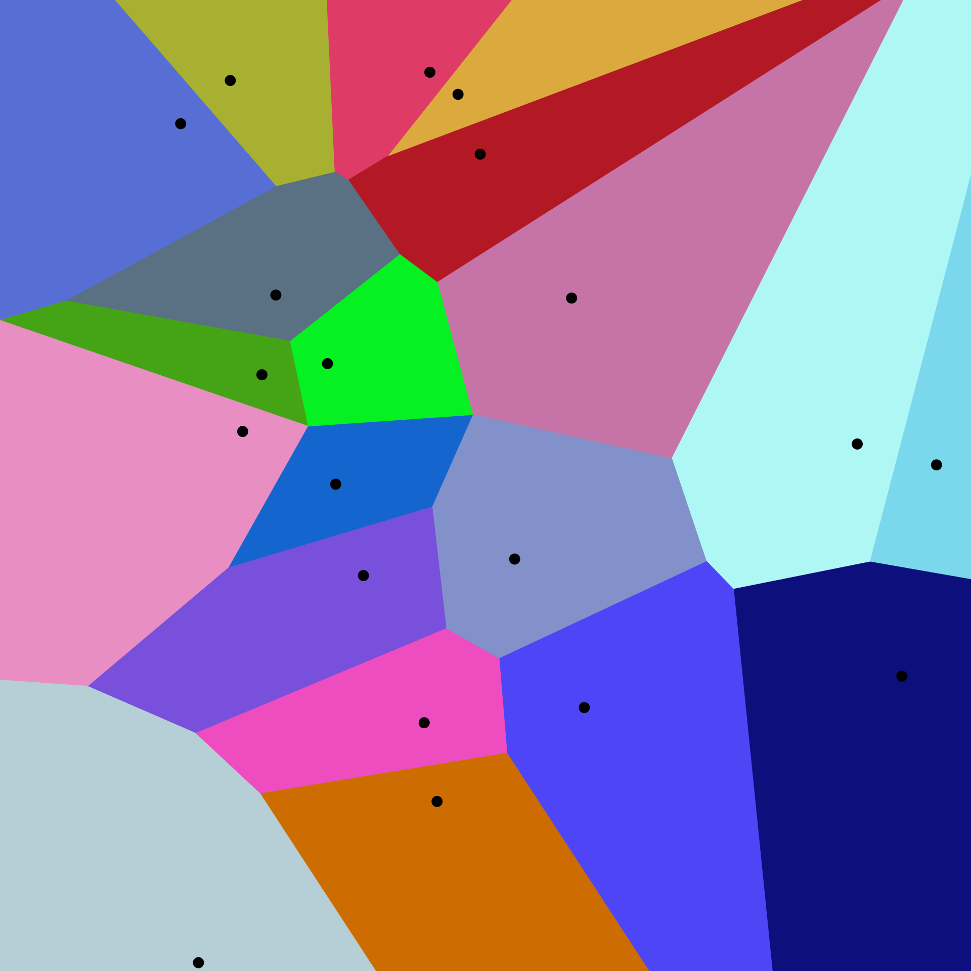
In order to determine which data points are closest to a given query point, the distance between the query point and the other data points will need to be calculated. These distance metrics help to form decision boundaries, which partitions query points into different regions. You commonly will see decision boundaries visualized with Voronoi diagrams. [1]

\begin{aligned} \left(\sum_{i=1}^n |x_i - y_i|^p)\right)^{1/p} \end{aligned}\nonumber

Euclidean distance (p=2)
Manhattan distance (p=1)
Minkowski distance
Hamming distance

Voronoi diagrams:

Euclidean distance (p=2)

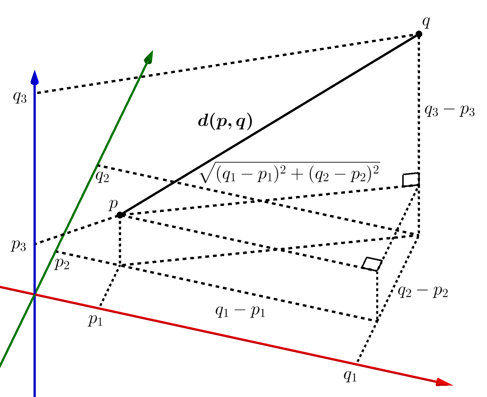
This is the most commonly used distance measure, and it is limited to real-valued vectors. Using the below formula, it measures a straight line between the query point and the other point being measured. [3]

\begin{gather*} d(p,q) = \sqrt{\sum_{i=1}^{n}(p_i - q_i)^2} \\\\ p, q: \ \text{two points in Euclidean n-space} \\ q_i, p_i: \ \text{Euclidean vectors, starting from the origin of the space (initial point)} \\ n: \ \text{n-space} \end{gather*}

Higher dimensions

Squared Euclidean distance

In many applications, and in particular when comparing distances, it may be more convenient to omit the final square root in the calculation of Euclidean distances, as the two distances are proportional. The value resulting from this omission is the square of the Euclidean distance, and is called the squared Euclidean distance

A cone, the graph of Euclidean distance from the origin in the plane	A paraboloid, the graph of squared Euclidean distance from the origin

Defining K

The k value in the k-NN algorithm defines how many neighbors will be checked to determine the classification of a specific query point. For example, if k=1, the instance will be assigned to the same class as its single nearest neighbor. Defining k can be a balancing act as different values can lead to overfitting or underfitting. [1]

Lower values of k
- has high variance, but low bias
- good at capturing fine-grained patterns [2]
- may overfit, i.e sensitive to random noise [2]
- excellent for training data, not that good for new data [2]
larger values of k
- may lead to high bias and lower variance
- stable predictions by averaging over large samples [2]
- may underfit, i.e. fail to cptrure important regularities [2]
- not good fot tarining data, not good for new data [2]

The choice of k will largely depend on the input data as data with more outliers or noise will likely perform better with higher values of k. Overall, it is recommended to have an odd number for k to avoid ties in classification, and cross-validation tactics can help you choose the optimal k for your dataset. [1]

Applications of k-NN in machine learning

The k-NN algorithm has been utilized within a variety of applications, largely within classification. Some of these use cases include: [1]

- Data preprocessing: Datasets frequently have missing values, but the KNN algorithm can estimate for those values in a process known as missing data imputation.

- Recommendation Engines: Using clickstream data from websites, the KNN algorithm has been used to provide automatic recommendations to users on additional content. This research (link resides outside of ibm.com) shows that the a user is assigned to a particular group, and based on that group’s user behavior, they are given a recommendation. However, given the scaling issues with KNN, this approach may not be optimal for larger datasets.

- Finance: It has also been used in a variety of finance and economic use cases. For example, one paper (PDF, 391 KB) (link resides outside of ibm.com) shows how using KNN on credit data can help banks assess risk of a loan to an organization or individual. It is used to determine the credit-worthiness of a loan applicant. Another journal (PDF, 447 KB)(link resides outside of ibm.com) highlights its use in stock market forecasting, currency exchange rates, trading futures, and money laundering analyses.

- Healthcare: KNN has also had application within the healthcare industry, making predictions on the risk of heart attacks and prostate cancer. The algorithm works by calculating the most likely gene expressions.

- Pattern Recognition: KNN has also assisted in identifying patterns, such as in text and digit classification (link resides outside of ibm.com). This has been particularly helpful in identifying handwritten numbers that you might find on forms or mailing envelopes.

Advantages and disadvantages of the KNN algorithm

Advantages: [1]

Easy to implement: Given the algorithm’s simplicity and accuracy, it is one of the first classifiers that a new data scientist will learn.
Adapts easily: As new training samples are added, the algorithm adjusts to account for any new data since all training data is stored into memory.
Few hyperparameters: KNN only requires a k value and a distance metric, which is low when compared to other machine learning algorithms.

Disadvantages: [1]

Does not scale well: Since KNN is a lazy algorithm, it takes up more memory and data storage compared to other classifiers. This can be costly from both a time and money perspective. More memory and storage will drive up business expenses and more data can take longer to compute. While different data structures, such as Ball-Tree, have been created to address the computational inefficiencies, a different classifier may be ideal depending on the business problem.
Curse of dimensionality: The KNN algorithm tends to fall victim to the curse of dimensionality, which means that it doesn’t perform well with high-dimensional data inputs. This is sometimes also referred to as the peaking phenomenon (PDF, 340 MB) (link resides outside of ibm.com), where after the algorithm attains the optimal number of features, additional features increases the amount of classification errors, especially when the sample size is smaller.
Prone to overfitting: Due to the “curse of dimensionality”, KNN is also more prone to overfitting. While feature selection and dimensionality reduction techniques are leveraged to prevent this from occurring, the value of k can also impact the model’s behavior. Lower values of k can overfit the data, whereas higher values of k tend to “smooth out” the prediction values since it is averaging the values over a greater area, or neighborhood. However, if the value of k is too high, then it can underfit the data.

References

Wiki https://en.wikipedia.org/wiki/Euclidean_distance