
Multi-Agent Cooperative Driving in HighwayEnv
Department of ECE, University of Toronto
- Jia Shu (Forrest) Zhang, [email protected]
- Yan Zhang, [email protected]
- JiaXuan Zhao, [email protected]
Github Repo: highway-agent-401
Abstract
The Canadian Motor Vehicle Traffic Collision Statistics 2022 Report [1] highlighted a concerning rise in motor vehicle fatalities, reaching 1,931, up 6% from 2021. Addressing these issues necessitates advancements in traffic management and the development of intelligent auto-driving systems. In this report, we present our project on traffic management in complex driving scenarios using reinforcement learning. Our focus is on developing multi-agent reinforcement learning (MARL) techniques within simulated environments based on HighwayEnv [2]. The primary objective is to enable multiple vehicles to navigate cooperatively through intricate road networks, ensuring safety and efficiency by avoiding collisions and minimizing congestion.
1 Introduction
Driving is one of most important part of daily life in modern society, but the number of people who die in traffic accidents each year remains alarmingly high. According to the Canadian Motor Vehicle Traffic Collision Statistics 2022 Report [1], the number of motor vehicle fatalities increased to 1,934 a rise from 2021. Serious injuries and total injuries also saw an increase of compared to 2021 . To reduce fatalities and enhance public safety, improvements in traffic management and intelligent auto-driving techniques are essential.
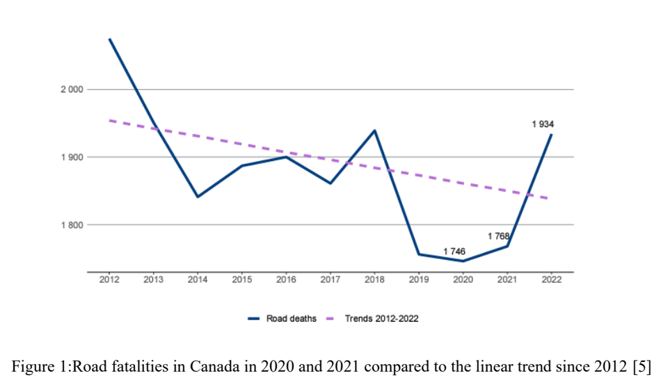
Managing traffic flow in complex driving scenarios, such as highways with multiple entry and exit points, intersections, and roundabouts, presents significant challenges in ensuring safety and efficiency. Traditional traffic management systems often rely on heuristic-based approaches, which can struggle to adapt to dynamic and unpredictable environments. This project aims to develop and evaluate multi-agent reinforcement learning (MARL) techniques to address these challenges. We focus on a simulated environment, Highway-401, which combines highway, merging, intersection, and roundabout scenarios from HighwayEnv [2] into one. Leveraging the capabilities of deep reinforcement learning (RL), our goal is to enable multiple vehicles to operate cooperatively, navigating through complex road networks while avoiding collisions and minimizing congestion.
2 Preliminaries
The tasks and milestones are divided into four parts: set up single agent environment, implement single agent algorithms, set up multi agent environment, and implement multi agent algorithms. We will use a simulated environment called Highway-401 to simulate one or more cars(agents) running on the highway. The detail for this environment is shown in Table 1. We will combine the normal highway with several situations, including merge, roundabout, intersection. Although each situation has its unique definition, they have several general states and actions.
Observation Type: Three primary observation types were tested to provide diverse perspectives on the environment. (1) Kinematics: The KinematicObservation is a array that describes a list of V nearby vehicles by a set of features of size, listed in the “features” configuration field. Kinematics data is crucial for understanding the dynamics of the environment and for making decisions based on the movement and behavior of surrounding vehicles. (2) OccupancyGrid: The OccupancyGridObservation is a array, that represents a grid of shape discretizing the space ( ) around the ego-vehicle in uniform rectangle cells. Each cell in the grid indicates whether it is occupied, providing a spatial map that helps the agent understand the layout and traffic density. (3) GrayScale: The GrayscaleObservation is a S grayscale image of the scene, where W, H are set with the observation shape parameter, and stack(S) are images from previous time frames. This type is particularly useful for tasks that require visual recognition, such as lane detection or identifying road markings. The grayscale representation allows the agent to perceive the environment in a way like a camera sensor, facilitating the use of computer vision techniques. State to Observation Mapping: The state of the environment is mapped to observations that the agent can use for decision-making. We chose GrayScale for our project because it provides a more comprehensive representation of the environment. Unlike Kinematics, which only detects other vehicles without providing information about the road orientation, GrayScale captures visual details of the entire scene, including road boundaries and markings. Additionally, while OccupancyGrid focus solely on spatial occupancy without considering vehicle orientation, GrayScale allows us to see the road’s layout and features, accommodating various road orientations. Actions: The HighwayEnv environments have two types of actions: “ContinuousAction” and “DiscreteMetaAction”. ContinuousAction contains continuous values that control the acceleration and steering of the car. DiscreteMetaAction are high level actions such as “LANE_LEFT” that are translated to low level ContinuousAction .
Rewards: In the Highway-401 environment, we focus on two primary objectives: ensuring vehicles progress quickly while respecting speed limits and avoiding collisions. Additionally, vehicles are rewarded for maintaining their position in the right lane.
The reward function for the vehicle’s speed can be calculated as follows:
where:
is the speed limit, is the vehicle’s speed, (controls the width of the Gaussian curve), (penalty factor controlling how quickly the penalty increases), (the fixed reward magnitude).
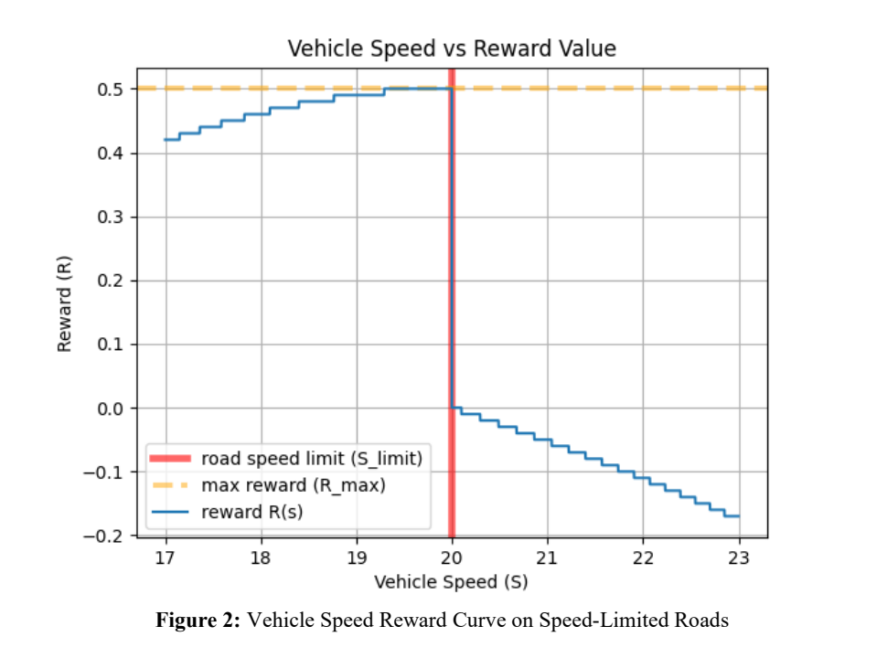
Table 1: States, Actions, and Rewards in Highway-401
| Aspect | Category | Description |
|---|---|---|
| States | GrayScale | W H S. W,H are set with the observation_shape parameter, and stack(S) is images from previous time frames. |
| Actions | DiscreteMetaAction | Integer {0: “LANE_LEFT”, 1: “IDLE”, 2: “LANE_RIGHT”, 3: “FASTER”, 4: “SLOWER”} |
| Rewards | Collision reward | The reward received when colliding with a vehicle. |
| Right lane reward | 1 The reward received when driving on the right-most lanes, linearly mapped to zero for other lanes. | |
| High speed reward | 0.5 When the vehicle’s speed is close to the road speed limit, it earns the full reward; the reward decreases when the speed is below the limit and becomes negative when the speed exceeds the limit. The non-linear speed reward equation is defined in Equation 1, and a sample speed reward graph is shown in Figure 2. | |
| Merging speed reward | -0.5 The reward related to altruistic penalty if any vehicle on the merging lane has a low speed. |
3 Solution via Classical RL Algorithms
We considered Q-Learning to a shortened highway environment. For the states and actions, we directly used the default “Kinematics” observation type and “DiscreteMetaAction” type from HighwayEnv to construct our state-action value functions. The types are described in Table 1.
We anticipated that classical RL approaches without policy and value approximation would not be very effective for driving tasks because the states would need to include continuous information on the position, velocity, and direction of all other vehicles.
With tabular approaches, the smallest variation in a neighboring vehicle can result in a new entry, making it infeasible to cover all cases. Practically speaking, our agent does not need all the information in the continuous features (e.g., the exact position of another car). On a basic level, it only needs to know if a neighboring car is close enough to require additional navigation to avoid collisions by changing lanes or speed.
Nonetheless, we implemented a basic Q-learning training loop to test our hypothesis. For each run, we trained the agent for 2000 episodes followed by 10 test episodes. A test episode is considered “passing” if the agent does not collide with another car. The hyperparameters and pass rates are described in Table 2.
Table 2: Q-Learning Results for simplified highway environment
| Run | alpha | gamma | epsilon | epsilon_decay | epsilon_min | Pass Rate |
|---|---|---|---|---|---|---|
| Run 1 | 0.1 | 0.99 | 1.0 | 0.995 | 0.1 | |
| Run 2 | 0.1 | 0.99 | 1.0 | 0.999 | 0.1 | |
| Run 3 | 0.05 | 0.99 | 1.0 | 0.999 | 0.1 |
4 Deep RL Implementation
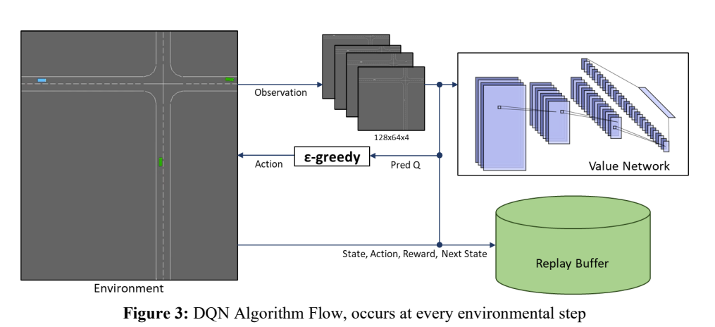
We choose to use deep Q-networks (DQN) for the car agents. The DQN agent accepts a stack of GrayScale images that captures the timelapse of the environment centered on the observing car agent. The DQN outputs the action-state values for each of the 5 DiscreteMetaActions. The network architecture and algorithm are described in Table 3 and Figure 3 respectively. The agent contains a memory replay buffer and two CNNs for the value and target networks.
Algorithm
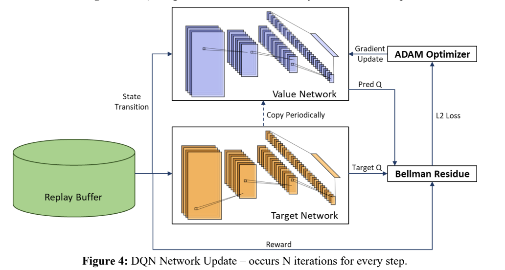
In each environment step, the time-lapsed grayscale images are passed into the value network. The agent then selects the action from the predicted values using a -greedy policy. The state transition and rewards are then recorded in the replay buffer, which follows a first in first out policy. After each step, the agent updates the networks with the replay buffer (fig 4). It randomly samples a batch of transitions from the buffer and passes the observations to the value and target networks. The agent then collects the prediction and target Q values and calculates the squared Bellman residue for the L2 loss. The loss is passed to the ADAM optimizer to update the value network. Periodically, the weights of the value network are copied into the target network.
Table 3: CNN Architecture
| Layer | Input Channels | Output Channels | Kernel Size | Stride |
|---|---|---|---|---|
| Conv2d | 4 | 16 | ||
| Conv2d | 16 | 32 | ||
| Conv2d | 32 | 64 | ||
| Linear | 8192 | 5 | N/A | N/A |
Multi-Agent
For the multi-agent scenario, we pass the observations in a loop into the networks for each agent. The colour of the observing car is also changed to a unique colour to distinguish it from other agentcontrolled cars.
Implementation
We implemented our agents using the rl-agent repo, which implements common reinforcement learning components such as Q-networks and memory buffers in PyTorch. These components are instantiated by specifying their parameters in JSON files.
5 Numerical Experiments
In this section, we detail the experimental setup and results for training a Deep Q-Network (DQN) agent in a multi-agent driving environment, referred to as the Highway-401 environment. This environment consists of two controllable vehicles, which interact within a simulated road scenario involving multiple agents.
5.1. Experimental Setup
The DQN agent was trained over a total of 2500 episodes. We fixed several hyperparameters across all experiments to maintain consistency and focus our analysis on the impact of varying key parameters. The fixed hyperparameters included:
- Episodes: 2500
- Batch size: 32
- Network iterations per step: 1
- Target network copy interval: 50 steps
- Memory buffer size: 15000
We conducted a series of experiments where we varied the discount factor , epsilon decay ratio , and learning rate (lr). These parameters are critical to the learning process and were adjusted to observe their effect on the agents’ performance. The specific values used for these parameters are summarized in Table 4.
Table 4: Summary of parameter variations across different experiments.
| Experiment | |||
|---|---|---|---|
| 0.8 | 5000 | ||
| 0.95 | 2500 | ||
| 0.95 | 2500 | ||
| 0.95 | 5000 | ||
| 0.95 | 5000 |
5.2. Training Results
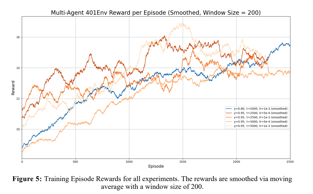
Figure 5 shows the training reward per episode of each experiment with moving average smoothing. Due to the epsilon greedy algorithm, the raw training rewards are extremely noisy as a random move can cause a vehicle to crash and end the episode. We applied smoothing to show the gradual increase of the rewards over time. For the experiments with , the reward plateaus around episode 1500 . For the experiment with , the reward plateaus around episode 2300 .
5.3. Evaluation
Post-training, we evaluated our train agents by testing each agent in the Highway-401 Env 10 times. The environment consists of 3 main sections in series: merge, intersection, and roundabout. Table 5 shows the percentage of runs for each experiment that cleared each section with at least 1 car. Table 5: Pass rates for each experiment for each obstacle in the Highway-401 environment,
| Merge | Intersection | Roundabout | |
|---|---|---|---|
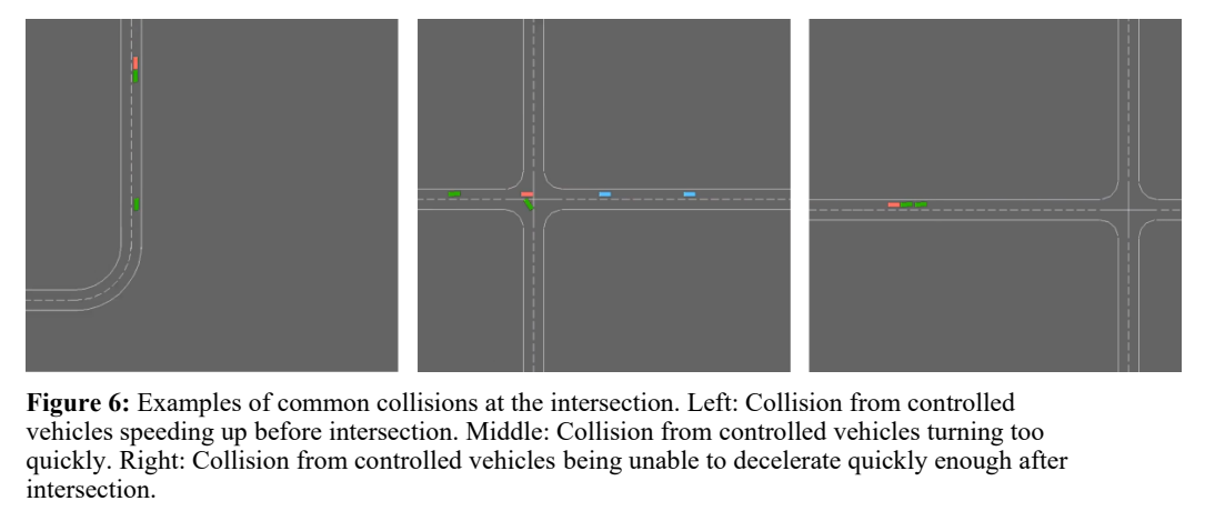
The majority of crashes occurs around the intersection component of the environment. We noticed that the controlled vehicles would rapidly speed up and attempt the intersection at a high speed. Fig X. depicts common scenarios for collisions at the intersection.
We expected the agent to learn to stop or slow down before the intersection and wait for a safe opportunity to pass, but we hypothesis that the speed reward in our environment is interfering with the agent’s ability to learn to slow down.
For video demonstrations of our test runs, please visit this link.
6 Answer Research Questions
6.1 Impact of Environment Action Space and Rewards
In the first version of the Highway-401 environment, we attempted to change the action space of the vehicles to a continuous action space, as it is closer to real-world scenarios. However, introducing continuous actions posed significant challenges during the training process. In the HighwayEnv environment, continuous action vehicles do not support the road planning feature and can move in any direction. As a result, vehicles often drove off-road and circled aimlessly, unable to reach their destinations even without non-player cars present. Due to these issues, we reverted to a discrete action space. Please see Appendix B for the training plots and pass rate table.
In addition to exploring the action space, we also optimized the reward system to improve the training process. Initially, vehicles would maintain high speeds when entering intersections because they were rewarded for high speeds on highways and merging roads. This caused vehicles to have insufficient time to slow down, leading to frequent collisions at intersections and complicating the training. To address this, we optimized the speed reward system using a non-linear function to compute rewards. When the vehicle’s speed is very close to the speed limit, it earns the full reward; the reward decreases when the speed is below the limit and becomes negative when the speed exceeds the limit. After implementing this change and setting speed limits at intersections, the agents learned to slow down vehicles when entering intersection roads.
6.2 Multi-Agent vs Single-Agent
Training reinforcement learning agents in a multi-agent environment introduces unique challenges compared to a single-agent setup. One significant challenge is the application of an epsilon-greedy policy, which is often used to balance exploration and exploitation. In a multi-agent setting, this policy is applied to all agents simultaneously, increasing the likelihood of suboptimal actions. For instance, an agent might choose an exploratory action that results in a collision, prematurely ending the episode and reducing the overall quality of the training data.
However, a key benefit is the ability to leverage shared experiences across agents. When agents operate in a shared environment, the experiences of one agent can be utilized to train the value network that is common to all agents. This shared learning approach can lead to more robust value estimates, as the network can aggregate and generalize from the diverse experiences of multiple agents, potentially leading to more efficient learning and better overall performance.
6.3 Parameter Sensitivity
In this study, we evaluated the performance of our trained agents in the Highway-401 environment by testing different parameter configurations. The environment includes three main sections: merge, intersection, and roundabout. Our goal was to understand the impact of varying the discount factor , target network update frequency , and learning rate (lr) on the agents’ ability to navigate these sections successfully.
6.3.1 Discount Factor ( )
Impact: The discount factor determines how much future rewards are valued compared to immediate rewards.
Observations: Increasing from 0.8 to 0.95 generally improved performance across all sections. Specifically, a higher resulted in better performance at intersections, where valuing future rewards (such as avoiding collisions) is critical.
6.3.2 Target Network Update Frequency ( )
Impact: This parameter controls how frequently the target network is updated, influencing the agent’s ability to adapt to changes.
Observations: Lowering to 2500 steps improved intersection performance, suggesting that more frequent updates help the agent adapt better to dynamic environments. However, steps still provided stable performance, indicating some flexibility in this parameter.
6.3.3 Learning Rate (Ir)
Impact: The learning rate determines the step size during gradient descent, affecting the stability and speed of learning.
Observations: A lower learning rate (5e-4) generally resulted in better performance at intersections and roundabouts, suggesting that smaller steps allow the agent to learn more stable policies. Interestingly, the highest merge section success rate ( ) was achieved with a higher learning rate (1e-3), indicating that faster learning can benefit simpler navigation tasks.
7 Conclusions
During this project, we explored various deep reinforcement learning algorithms for the customized Highway-401 environment. We encountered the complexities and challenges of managing traffic flow in dynamic and unpredictable multi-agent settings. Our experiments with both continuous and discrete action spaces underscored the importance of selecting appropriate action representations for effective training. Additionally, optimizing the reward system was crucial for guiding the agents towards desired behaviours, such as slowing down at intersections to avoid collisions.
For future improvements, several areas can be explored:
- Optimizing Memory Buffer: The memory buffer should avoid storing all transitions indiscriminately. Balancing the buffer between different states and either partitioning it based on transition types or assigning priorities to transitions can improve efficiency.
- Enhanced Neural Networks: Experimenting with deeper and more complex neural networks could potentially enhance performance. Incorporating batch normalization layers, skip connections, and more advanced training techniques like dropout or cutout could further refine the models.
- Policy Improvements: Trying off-policy methods and collecting datasets to leverage CUDA more effectively could lead to significant gains in computational efficiency and training speed.
- Environment Complexity: Making the environment more complex by adding stop signs, traffic lights, and more cooperative rewards would provide a more realistic and challenging setting for the agents to learn and operate within.
References
[1] T. Canada, “Canadian Motor Vehicle Traffic Collision Statistics: 2022,” Transport Canada, 2 5 2024. [Online]. Available: https://tc.canada.ca/en/road-transportation/statistics-data/canadian-motor-vehicle-traffic-collision-statistics-2022.
[2] L. Edouard, “highway-env,” 2018. [Online]. Available: https://highway-env.farama.org/.
[3] A. H. A. G. K. E. D. Antonin Raffin, “Stable-Baselines3,” 2021. [Online]. Available: https://stable-baselines3.readthedocs.io/.
[4] L. Edouard, “rl-agents,” 2018. [Online]. Available: https://github.com/eleurent/rl-agents.
[5] I. T. Form, “Road Safety Country Profiles Canada 2023,” 2023. [Online]. Available: https://www.itf-oecd.org/sites/default/files/canada-road-safety.pdf.